Section11.1Introduction to Multivariable Functions
Definition11.1.1.Function of Two Variables.
Let \(D\) be a subset of \(\mathbb{R}^2\text{.}\) A function \(f\) of two variables is a rule that assigns each pair \((x,y)\) in \(D\) a value \(z=f(x,y)\) in \(\mathbb{R}\text{.}\)\(D\) is the domain of \(f\text{;}\) the set of all outputs of \(f\) is the range.
The domain is not specified, so we take it to be all possible pairs in \(\mathbb{R}^2\) for which \(f\) is defined. In this example, \(f\) is defined for all pairs \((x,y)\text{,}\) so the domain \(D\) of \(f\) is \(\mathbb{R}^2\text{.}\)
The output of \(f\) can be made as large or small as possible; any real number \(r\) can be the output. (In fact, given any real number \(r\text{,}\)\(f(0,-r)=r\text{.}\)) So the range \(R\) of \(f\) is \(\mathbb{R}\text{.}\)
The domain is all pairs \((x,y)\) allowable as input in \(f\text{.}\) Because of the square root, we need \((x,y)\) such that \(0\leq1-\frac{x^2}9-\frac{y^2}4\text{:}\)
The above equation describes an ellipse and its interior as shown in Figure 11.1.5. We can represent the domain \(D\) graphically with the figure; in set notation, we can write \(D = \{(x,y)|\,\frac{x^2}9+\frac{y^2}4 \leq 1\}\text{.}\)
The ellipse \(\frac{x^2}{9}+\frac{y^2}{4}=1\) is plotted in the \(xy\) plane. It is centered at the origin, with intercepts at \((\pm 3,0)\) and \((0,\pm 2)\text{.}\) The interior of the ellipse is shaded, to illustrate the domain of \(f(x,y) = \sqrt{1-\frac{x^2}{9}-\frac{y^2}{4}}\text{.}\)
The range is the set of all possible output values. The square root ensures that all output is \(\geq 0\text{.}\) Since the \(x\) and \(y\) terms are squared, then subtracted, inside the square root, the largest output value comes at \(x=0\text{,}\)\(y=0\text{:}\)\(f(0,0) = 1\text{.}\) Thus the range \(R\) is the interval \([0,1]\text{.}\)
Subsection11.1.1Graphing Functions of Two Variables
The graph of a function \(f\) of two variables is the set of all points \(\big(x,y,f(x,y)\big)\) where \((x,y)\) is in the domain of \(f\text{.}\) This creates a surface in space.
About two dozen points are plotted in space, along with a set of three-dimensional coordinate axes. The location of the points can be better observed by rotating the figure, but the precise arrangement of the points is unimportant. The main observation is that these points all lie on the surface plotted in the next image.
A three-dimensional plot the surface given by a graph \(z=f(x,y)\text{.}\) The surface is a bell-shaped hill, with its peak at \((0,0,1)\) on the \(z\) axis. There is rotational symmetry about the \(z\) axis, and as the suface descends, it flattens out and tapers off toward the \(xy\) plane.
One can begin sketching a graph by plotting points, but this has limitations. Consider Figure 11.1.6(a) where 25 points have been plotted of \(f(x,y) = \frac1{x^2+y^2+1}\text{.}\) More points have been plotted than one would reasonably want to do by hand, yet it is not clear at all what the graph of the function looks like. Technology allows us to plot lots of points, connect adjacent points with lines and add shading to create a graph like Figure 11.1.6(b) which does a far better job of illustrating the behavior of \(f\text{.}\)
While technology is readily available to help us graph functions of two variables, there is still a paper-and-pencil approach that is useful to understand and master as it, combined with high-quality graphics, gives one great insight into the behavior of a function. This technique is known as sketching level curves.
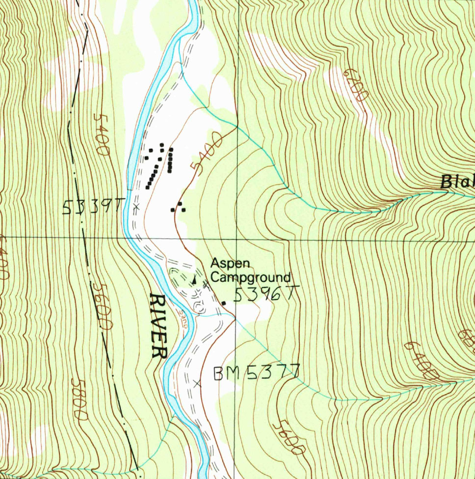
It may be surprising to find that the problem of representing a three dimensional surface on paper is familiar to most people (they just don’t realize it). Topographical maps, like the one shown in Figure 11.1.7, represent the surface of Earth by indicating points with the same elevation with contour lines. The elevations marked are equally spaced; in this example, each thin line indicates an elevation change in 50ft increments and each thick line indicates a change of 200ft. When lines are drawn close together, elevation changes rapidly (as one does not have to travel far to rise 50ft). When lines are far apart, such as near “Aspen Campground,” elevation changes more gradually as one has to walk farther to rise 50ft.
An excerpt from a topographical map of Chrome Mountain in Montana. The map illustrates the concept of contour lines through its use of lines of elevation. There is a river that runs through the middle of the map, from top to bottom. To the right of the river, the lines of elevation are more spread out, indicating that the land is more gently-sloped in this region, which includes an area marked as “Aspen Campground”.
Near the left and right edges of the map, the lines of elevation are much closer together, which indicates that these regions consist of steeply-sloped mountainsides.
Figure11.1.7.A topographical map displays elevation by drawing contour lines, along with the elevation is constant. USGS 1:24000-scale Quadrangle for Chrome Mountain, MT 1987.
Given a function \(f(x,y)\text{,}\) we can draw a “topographical map” of the graph \(z=f(x,y)\) by drawing level curves (or, contour lines). A level curve at \(z=c\) is a curve in the \(xy\)-plane such that for all points \((x,y)\) on the curve, \(f(x,y) = c\text{.}\)
When drawing level curves, it is important that the \(c\) values are spaced equally apart as that gives the best insight to how quickly the “elevation” is changing. Examples will help one understand this concept.
Let \(f(x,y) = \sqrt{1-\frac{x^2}9-\frac{y^2}4}\text{.}\) Find the level curves of \(f\) for \(c=0\text{,}\)\(0.2\text{,}\)\(0.4\text{,}\)\(0.6\text{,}\)\(0.8\) and \(1\text{.}\)
Consider first \(c=0\text{.}\) The level curve for \(c=0\) is the set of all points \((x,y)\) such that \(0=\sqrt{1-\frac{x^2}9-\frac{y^2}4}\text{.}\) Squaring both sides gives us
an ellipse centered at \((0,0)\) with horizontal major axis of length 6 and minor axis of length 4. Thus for any point \((x,y)\) on this curve, \(f(x,y) = 0\text{.}\)
The level curves are shown in Figure 11.1.9(a). Note how the level curves for \(c=0\) and \(c=0.2\) are very, very close together: this indicates that \(f\) is growing rapidly along those curves.
This plot, in the \(xy\) plane, illustrates several level curves for the function \(f(x,y) = \sqrt{1-\frac{x^2}{9}-\frac{y^2}{4}}\text{.}\) The level “curve” \(c=1\) is a single point: the origin \((0,0)\text{.}\) The other level curves form a family of concentric ellipses centered about the origin. The largest ellipse is the boundary of the domain of \(f\text{,}\) given by \(\frac{x^2}{9}+\frac{y^2}{4}=1\text{.}\) Level curves near the boundary are close together, while those nearer to the origin are further apart. This illustrates the fact that the surface is relative flat near the top, while it becomes steeply-sloped along its sides.
The surface given by the graph \(z=\sqrt{1--\frac{x^2}{9}-\frac{y^2}{4}}\) is plotted. Its shape is that of an elliptical dome, with its peak on the \(z\) axis at the point \((0,0,1)\text{.}\) The bottom of the dome lies in the \(xy\) plane, and its intersection with this plane is an ellipse. Near the top, the surface is relatively flat, but the sides become close to vertical near the \(xy\) plane.
In Figure 11.1.9(b), the curves are drawn on a graph of \(f\) in space. Note how the elevations are evenly spaced. Near the level curves of \(c=0\) and \(c=0.2\) we can see that \(f\) indeed is growing quickly.
a circle centered at \(\big(1/(2c),1/(2c)\big)\) with radius \(\sqrt{1/(2c^2)-1}\text{,}\) where \(\abs{c}\lt 1/\sqrt{2}\text{.}\) The level curves for \(c=\pm 0.2,\,\pm 0.4\) and \(\pm0.6\) are sketched in Figure 11.1.11(a). To help illustrate “elevation,” we use thicker lines for \(c\) values near 0, and dashed lines indicate where \(c\lt 0\text{.}\)
In Figure 11.1.11(b) we see a graph of the surface. Note how the \(y\)-axis is pointing away from the viewer to more closely resemble the orientation of the level curves in Figure 11.1.11(a).
This plot in the \(xy\) plane shows several level curves for the function \(f(x,y) = \frac{x+y}{x^2+y^2+1}\text{.}\) The level curve \(c=0\) is the line \(y=-x\) passing through the origin. Above this line there is a family of nested, but not concentric, circles. The smallest circles are closest to the origin. These represent level curves for positive values of \(c\text{.}\) Across the line \(y=-x\) is another set of circles that is the mirror image of the first. These are the level curves for negative values of \(c\text{.}\)
The surface given by the graph \(z=\frac{x+y}{x^2+y^2+1}\) is plotted in three dimensions. For points that are far from the \(z\) axis, the surface lies close to the \(xy\) plane and is relatively flat. Near the origin, the surface rises sharply to a peak that lies above the line \(y=x\) in the \(xy\) plane. On the opposite side of the origin, the surface drops into a well that is the mirror image of the peak.
Seeing the level curves helps us understand the graph. For instance, the graph does not make it clear that one can “walk” along the line \(y=-x\) without elevation change, though the level curve does.
We extend our study of multivariable functions to functions of three variables. (One can make a function of as many variables as one likes; we limit our study to three variables.)
Let \(D\) be a subset of \(\mathbb{R}^3\text{.}\) A function \(f\) of three variables is a rule that assigns each triple \((x,y,z)\) in \(D\) a value \(w=f(x,y,z)\) in \(\mathbb{R}\text{.}\)\(D\) is the domain of \(f\text{;}\) the set of all outputs of \(f\) is the range.
As the domain of \(f\) is not specified, we take it to be the set of all triples \((x,y,z)\) for which \(f(x,y,z)\) is defined. As we cannot divide by \(0\text{,}\) we find the domain \(D\) is
\begin{equation*}
D = \{(x,y,z)\,|\,x+2y-z\neq 0\}\text{.}
\end{equation*}
We recognize that the set of all points in \(\mathbb{R}^3\) that are not in \(D\) form a plane in space that passes through the origin (with normal vector \(\la 1,2,-1\ra\)).
We determine the range \(R\) is \(\mathbb{R}\text{;}\) that is, all real numbers are possible outputs of \(f\text{.}\) There is no set way of establishing this. Rather, to get numbers near 0 we can let \(y=0\) and choose \(z \approx -x^2\text{.}\) To get numbers of arbitrarily large magnitude, we can let \(z\approx x+2y\text{.}\)
It is very difficult to produce a meaningful graph of a function of three variables. A function of one variable is a curve drawn in 2 dimensions; a function of two variables is a surface drawn in 3 dimensions; a function of three variables is a hypersurface drawn in 4 dimensions.
There are a few techniques one can employ to try to “picture” a graph of three variables. One is an analogue of level curves: level surfaces. Given \(w=f(x,y,z)\text{,}\) the level surface at \(w=c\) is the surface in space formed by all points \((x,y,z)\) where \(f(x,y,z)=c\text{.}\)
If a point source \(S\) is radiating energy, the intensity \(I\) at a given point \(P\) in space is inversely proportional to the square of the distance between \(S\) and \(P\text{.}\) That is, when \(S=(0,0,0)\text{,}\)\(I(x,y,z) = \frac{k}{x^2+y^2+z^2}\) for some constant \(k\text{.}\)
We can (mostly) answer this question using “common sense.” If energy (say, in the form of light) is emanating from the origin, its intensity will be the same at all points equidistant from the origin. That is, at any point on the surface of a sphere centered at the origin, the intensity should be the same. Therefore, the level surfaces are spheres.
Figure 11.1.15 gives a table of the radii of the spheres for given \(c\) values. Normally one would use equally spaced \(c\) values, but these values have been chosen purposefully. At a distance of 0.25 from the point source, the intensity is 16; to move to a point of half that intensity, one just moves out 0.1 to 0.35 — not much at all. To again halve the intensity, one moves 0.15, a little more than before.
Note how each time the intensity if halved, the distance required to move away grows. We conclude that the closer one is to the source, the more rapidly the intensity changes.
Compare the level curves of Exercises 21 and 22. How are they similar, and how are they different? Each surface is a quadric surface; describe how the level curves are consistent with what we know about each surface.